Measuring what an annotation really costs
Labelling is expensive: that was the everyday reality of my internship at Nricher, where an account manager reviews a sample of a thousand products in one to two days. The question here is the same one, isolated and measured: at a fixed annotation budget, which selection strategy makes the model improve fastest?
The protocol is deliberately strict. We start from ten randomly labelled examples, add batches of ten chosen by the strategy under test, retrain, and measure accuracy on a test set that is never touched. Every curve is the average of twenty independent draws — train/test split and seed set included — and every comparison is paired: the same seed gives random sampling and the tested strategy exactly the same starting point, which makes a Wilcoxon test meaningful.
Five strategies: random sampling; margin (the gap between the two most likely classes — the smaller it is, the more ambiguous the example); entropy of the predicted distribution; diversity (k-centres: the example farthest from everything already labelled); and margin then diversity, which shortlists ambiguous examples before picking ones far apart from each other.
Two hundred labels are almost enough
With 200 labels out of 1,257, that is 16% of the training set, the “margin then diversity” strategy reaches 0.960 accuracy, while training on all the labels tops out at 0.967. Random sampling stays at 0.926 on the same budget: that is thirty-four percentage points of error removed, for the same human work.
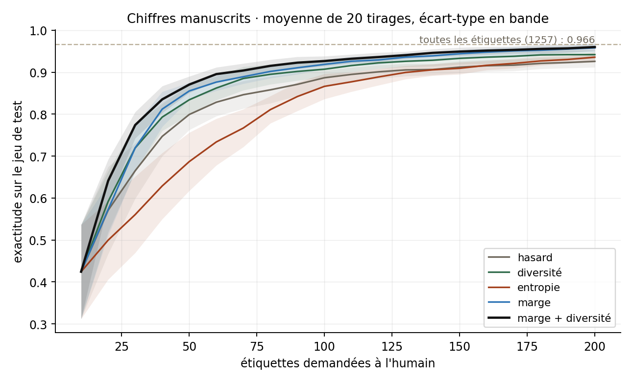
| Accuracy by label budget | 20 | 50 | 100 | 200 |
|---|---|---|---|---|
| margin + diversity | 0,641 | 0,871 | 0,927 | 0,960 |
| margin | 0,573 | 0,855 | 0,919 | 0,958 |
| diversity | 0,592 | 0,834 | 0,907 | 0,942 |
| random | 0,571 | 0,799 | 0,887 | 0,926 |
| entropy | 0,499 | 0,687 | 0,866 | 0,936 |
The gaps are significant at every budget for “margin then diversity” (p = 0.002 at twenty labels, p < 0.001 after that), and the conclusion survives a change of classifier: with a random forest, margin reaches 0.971 against 0.924 for random sampling at two hundred labels.
03 · What did not workEntropy, and problems that are too easy
Entropy does worse than random sampling at the start. At twenty labels it falls to 0.499 against 0.571 (p = 0.012); at fifty, 0.687 against 0.799 (p = 0.0002). The reason lies in the task: with ten classes and a barely trained model, the predicted distribution is flat almost everywhere, and entropy then selects the most confusing examples — often the most atypical ones, those you learn the least from. Margin, which only looks at the two best classes, aims far better.
A second limit, even more useful to know: on an easy problem, every strategy is equivalent. On the binary breast cancer diagnosis dataset, at one hundred and twenty labels, “margin then diversity” gives 0.974 and random sampling 0.967, while full training reaches 0.975. In other words, active learning only pays off when the task is hard or the classes are many. That is exactly the question to ask before offering it to a client.
04 · In the browserIs the model you are training the right one?
The sandbox calls no server: the multinomial logistic regression is rewritten in JavaScript, trained by gradient descent after each label, and evaluated on three hundred held-out images. It remained to check that it matches the reference implementation.
Over five games played automatically with the true labels, the browser model reaches 86.2% ± 1.3 at fifty labels and 89.1% ± 1.4 at seventy, against 85.5% ± 2.0 and 88.9% ± 1.7 for scikit-learn under the same conditions: less than one point apart from forty labels on. Below that, the browser model is even slightly better — its regularisation and limited number of iterations protect it when examples can be counted on one hand.