Two scenarios, one challenge
Smart meters record each household's electricity consumption every 30 minutes. Some readings were masked; the goal is to reconstruct them with the lowest possible mean absolute error (MAE), as part of an internal Kaggle challenge in the master's program.
| Scenario | Training | Test | Masked |
|---|---|---|---|
| Step A | 3,127 complete households | the same households | 30% |
| Step B | the same 3,127 households | 1,098 new households | 50% |
Consumption values are highly skewed, with long tails. Before any method, values outside [Q1 − 1.5·IQR, Q3 + 1.5·IQR] are clipped to the nearest quartile, so that outlier readings do not distort learning.
02 · The methodsFrom the simplest to the deepest
| Method | Principle |
|---|---|
| Nearest neighbor | copy the values of the closest training household, measured on the observed positions |
| GPU STL | trend + seasonality decomposition, rewritten in PyTorch |
| LSTM autoencoder | reconstruction of masked windows |
| PConv U-Net | 1D inpainting: convolutions only see observed values |
| Transformer | self-supervised masked imputation, trained on several GPUs |
STL, the winner, fits in a few lines. It starts from the nearest-neighbor imputation, then repeats 30 times:
- estimate the trend with a moving average, computed as a 1D convolution on GPU;
- estimate seasonality as the median residual at each phase of the cycle, for example daily (48 readings) or weekly (336);
- rebuild trend + seasonality and write the result back only at the missing positions.
The simplest method wins
Step A: same households, 30% masked
Step B: new households, 50% masked
GPU-accelerated STLtrend + seasonal decomposition
0.262 · 0.279
Nearest neighborcopy of the closest household
0.312 · 0.311
PConv U-Netpartial convolutions
0.327 · 0.333
Transformerself-supervised masking
0.331 · 0.344
LSTM autoencodermasked windows
0.335 · 0.356
The right inductive bias beats a big model
- The structure of the data. Electricity consumption is made of a trend plus daily and weekly cycles: exactly what STL assumes.
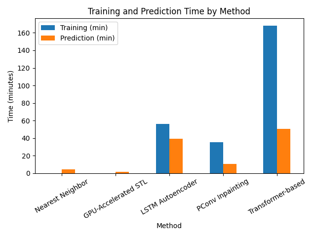
- The scale. 3,127 series of 12,864 points, tens of millions of time steps: high-capacity models converge poorly within a reasonable number of epochs.
- The budget. To fit on 4 GPUs, the deep models' depth, dimensions and sequence lengths had to be reduced, at the cost of their representational power.
Deep models remain an option, but they would need more compute, a lighter architecture or multi-stage pretraining to beat this baseline.